Moderation and Stratification

11
Author

Robin Donatello

Published

October 30, 2023

Setup

Code
library(tidyverse)  # general use
library(ggdist)     # for the "half-violin" plot (stat_slab)
library(ggpubr)     # ggscatter
library(scales)     # axes labeling
library(sjPlot)     # side by side barcharts with numbers
library(gtsummary)  # regression tables

pen <- palmerpenguins::penguins

Motivation - Ex. 1

Below are the admissions figures for Fall 1973 at UC Berkeley.

Table of admissions rates at UC Berkeley in 1973
Applicants Admitted
Total 12,763 41%
Men 8,442 44%
Women 4,321 35%

Is there evidence of gender bias in college admissions? Do you think a difference of 35% vs 44% is too large to be by chance?

Department specific data

The table of admissions rates for the 6 largest departments show a different story.
All Men Women
Department Applicants Admitted Applicants Admitted Applicants Admitted
A 933 64% 825 62% 108 82%
B 585 63% 560 63% 25 68%
C 918 35% 325 37% 593 34%
D 792 34% 417 33% 375 35%
E 584 25% 191 28% 393 24%
F 714 6% 373 6% 341 7%
Total 4526 39% 2691 45% 1835 30%

After adjusting for features such as size and competitiveness of the department, the pooled data showed a “small but statistically significant bias in favor of women”

Motivation Ex. 2

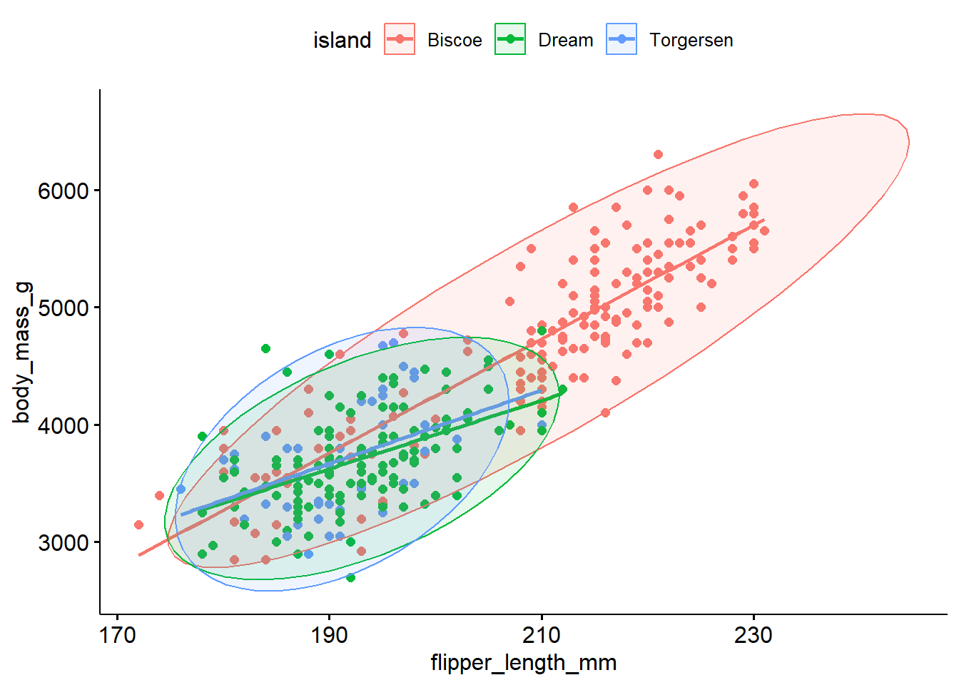
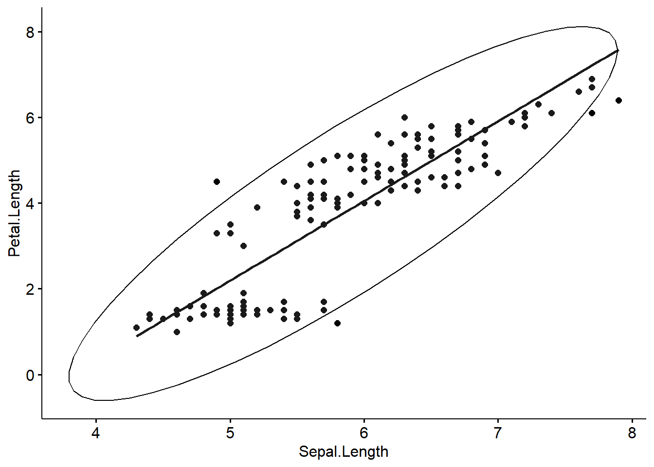
Can we predict penguin body mass from the flipper length?

ggscatter(pen, x="flipper_length_mm", y = "body_mass_g", add = "reg.line", 
          color = "island", ellipse = TRUE)

Probably, but the relationship between flipper length and body mass changes depending on what island they are found on.

Moderation

Moderation occurs when the relationship between two variables depends on a third variable.

  • The third variable is referred to as the moderating variable or simply the moderator.
  • The moderator affects the direction and/or strength of the relationship between the explanatory (\(x\)) and response (\(y\)) variable.
  • So we need a model that can allow for this difference in slope.
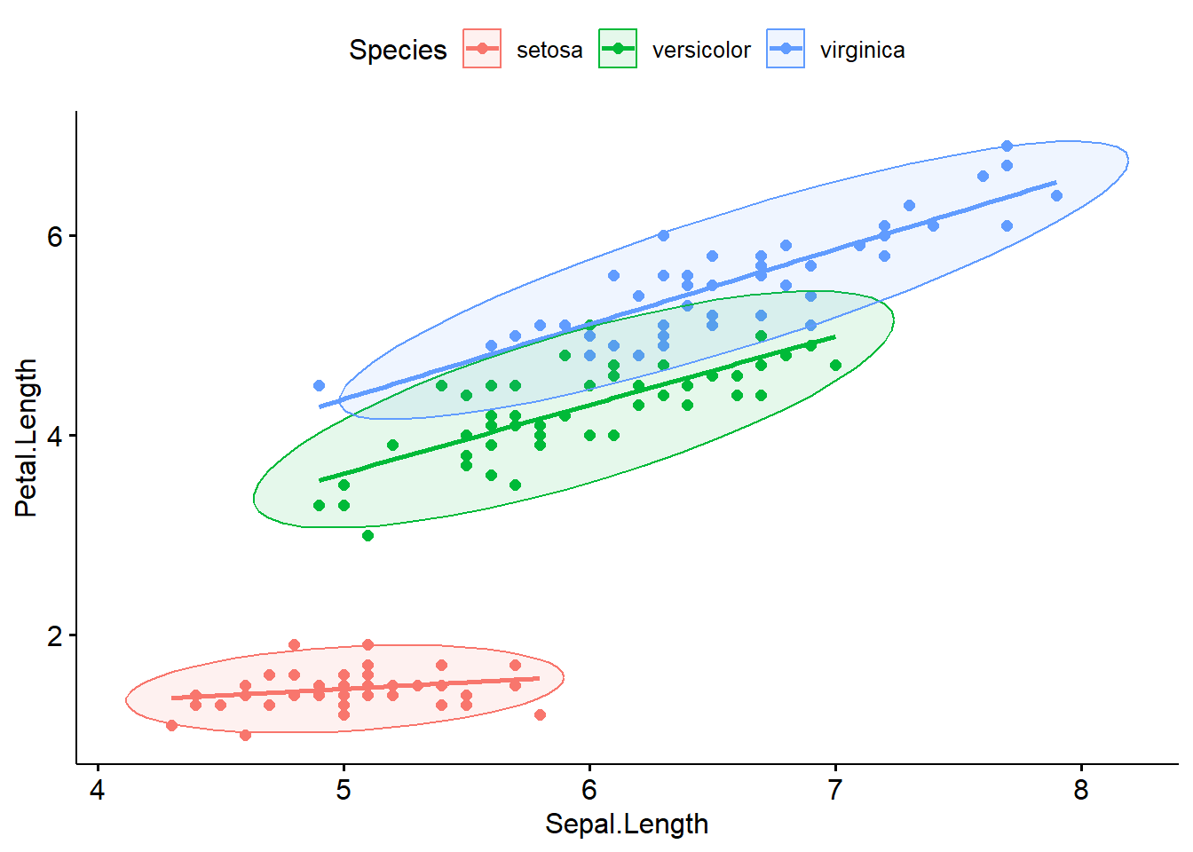
Stratification

Stratified models fit the regression equations (or any other bivariate analysis) for each subgroup of the population.

The mathematical model describing the relationship between body mass (\(Y\)), and flipper length (\(X\)) for each of the species separately would be written as follows:

\[ Y_{ib} \sim \beta_{0b} + \beta_{1b}*x_{i} + \epsilon_{ib} \qquad \epsilon_{ib} \sim \mathcal{N}(0,\sigma^{2}_{b})\] \[ Y_{id} \sim \beta_{0d} + \beta_{1d}*x_{i} + \epsilon_{id} \qquad \epsilon_{id} \sim \mathcal{N}(0,\sigma^{2}_{c}) \] \[ Y_{it} \sim \beta_{0t} + \beta_{1t}*x_{i} + \epsilon_{it} \qquad \epsilon_{it} \sim \mathcal{N}(0,\sigma^{2}_{t}) \]

where \(b, d, t\) indicates islands Biscoe, Dream and Torgersen respectively.

Stratification

Benefits
  • In each model, the intercept, slope, and variance of the residuals can all be different.
    • \(Y_{ij} \sim \beta_{0j} + \beta_{1j}*x_{i} + \epsilon_{ij} \qquad \epsilon_{ij} \sim \mathcal{N}(0,\sigma^{2}_{j})\)
  • This is the unique and powerful feature of stratified models.
Consequences
  • Each model is only fit on the amount of data in that particular subset.
  • Each model has 3 parameters that need to be estimated: \(\beta_{0}, \beta_{1}\), and \(\sigma^{2}\)
    • Total of 9 for the three models.
  • The more parameters that need to be estimated, the more data we need.

Identifying a Moderator

When testing a potential moderator, we are asking the question whether there is an association between two constructs, but separately for different subgroups within the sample.

We consider 3 scenarios demonstrating how a third variable can modify the relationship between the original two variables.

Significant –> Non-Significant

  • Significant relationship at bivariate level
    • We expect the effect to exist in the entire population
  • Within at least one level of the third variable the strength of the relationship changes
    • P-value is no longer significant within at least one subgroup

Non-Significant –> Significant

  • Non-significant relationship at bivariate level
    • We do not expect the effect to exist in the entire population
  • Within at least one level of the third variable the relationship becomes significant
    • P-value is now significant within at least one subgroup

Change in Direction of Association

  • Significant relationship at bivariate level
    • We expect the effect to exist in the entire population
  • Within at least one level of the third variable the direction of the relationship changes
    • Means change order, positive to negative correlation etc.

What to look for

ANOVA Chi-Square Regression
\(p\)-value, \(R^2\), means, density/boxplot \(p\)-value, col percents, side by side barcharts correlation coefficient (\(r\)), \(p\)-value, \(\beta\) coefficients, \(r\)-squared, scatterplot

Compare these values within each level of the potential moderator to the values in the overall model.

Example: ANOVA

Does sex modify the relationship between flipper length and species?

ggplot(pen, aes(x=flipper_length_mm, y=species, fill=species)) + 
      stat_slab(alpha=.5, justification = 0) + 
      geom_boxplot(width = .2,  outlier.shape = NA) + 
      geom_jitter(alpha = 0.5, height = 0.05) +
      stat_summary(fun="mean", geom="point", col="red", size=4, pch=17) + 
      theme_bw() + 
      labs(x="Flipper Length (mm)", y = "Species", title = "Overall") + 
      theme(legend.position = "none")

Gentoo have the larger flipper length by far, then Chinstrap is similar to Adelie but a little larger.

pen %>% select(flipper_length_mm, species, sex) %>% na.omit() %>%
ggplot(aes(x=flipper_length_mm, y=species, fill=species)) + 
      stat_slab(alpha=.5, justification = 0) + 
      geom_boxplot(width = .2,  outlier.shape = NA) + 
      geom_jitter(alpha = 0.5, height = 0.05) +
      stat_summary(fun="mean", geom="point", col="red", size=4, pch=17) + 
      theme_bw() + 
      labs(x="Flipper Length (mm)", y = "Species", title = "By Sex") + 
      theme(legend.position = "none") + 
  facet_wrap(~sex)

The pattern of distributions of flipper length by species seems the same for both sexes of penguin. Sex is likely not a moderator.

Example: ANOVA (cont.)

aov(pen$flipper_length_mm ~ pen$species) |> summary()
             Df Sum Sq Mean Sq F value Pr(>F)    
pen$species   2  52473   26237   594.8 <2e-16 ***
Residuals   339  14953      44                   
---
Signif. codes:  0 '***' 0.001 '**' 0.01 '*' 0.05 '.' 0.1 ' ' 1
2 observations deleted due to missingness
aov(pen$flipper_length_mm ~ pen$species) |> performance::r2()
# R2 for Anova Regression
       R2: 0.778
  adj. R2: 0.777

Highly significant p-value, \(R^2\) value of 0.77

by(pen, pen$sex, function(x) {
  p <- aov(x$flipper_length_mm ~ x$species) |> summary()
  r <- aov(x$flipper_length_mm ~ x$species) |> performance::r2()
  return(list=c(p, r))
  })
pen$sex: female
[[1]]
             Df  Sum Sq Mean Sq F value    Pr(>F)    
x$species     2 21415.6   10708  411.79 < 2.2e-16 ***
Residuals   162  4212.6      26                      
---
Signif. codes:  0 '***' 0.001 '**' 0.01 '*' 0.05 '.' 0.1 ' ' 1

$R2
       R2 
0.8356281 

$R2_adjusted
adjusted R2 
  0.8335988 

------------------------------------------------------------------------------------------------------------------------------------------------------ 
pen$sex: male
[[1]]
             Df  Sum Sq Mean Sq F value    Pr(>F)    
x$species     2 29098.4 14549.2  384.37 < 2.2e-16 ***
Residuals   165  6245.6    37.9                      
---
Signif. codes:  0 '***' 0.001 '**' 0.01 '*' 0.05 '.' 0.1 ' ' 1

$R2
       R2 
0.8232924 

$R2_adjusted
adjusted R2 
  0.8211504 

P-value still <.0001 in each group, \(R^2_{f}= 0.84, R^2_m = 0.82\). Same pattern.

Sex is not a modifier, the relationship between species and flipper length is the same within male and female penguins.

Example: Chi-Squared

Does gender modify the relationship between smoking and general health?

plot_xtab(addhealth$genhealth, addhealth$eversmoke_c, show.total = FALSE, margin = "row") + 
  ggtitle("Overall")

The proportion of smokers increases as the level of general health decreases.

addhealth %>%
  select(female_c, genhealth, eversmoke_c) %>% na.omit() %>% 
  group_by(female_c, genhealth) %>% 
  summarize(pct_smoke = mean(eversmoke_c == "Smoked at least once")) %>%
  ggplot(aes(x=genhealth, y = pct_smoke, fill = female_c)) + 
  geom_point(size=5, alpha=0.7, shape=21, stroke=2) +
  scale_y_continuous(limits = c(0, .8), labels = percent) + 
  theme_bw()

Mostly similar pattern within males and females

Example: Chi-Squared (cont)

chisq.test(addhealth$eversmoke_c, addhealth$genhealth)

    Pearson's Chi-squared test

data:  addhealth$eversmoke_c and addhealth$genhealth
X-squared = 30.795, df = 4, p-value = 3.371e-06

Highly significant p-value

by(addhealth, addhealth$female_c, function(x) chisq.test(x$eversmoke_c, x$genhealth))
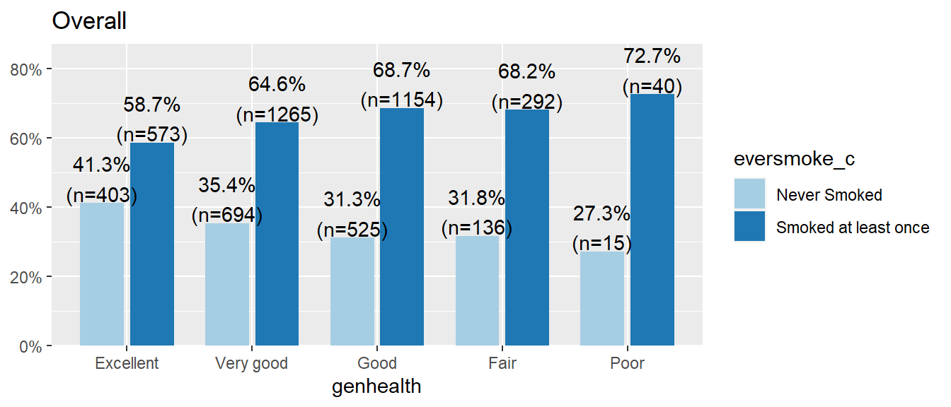
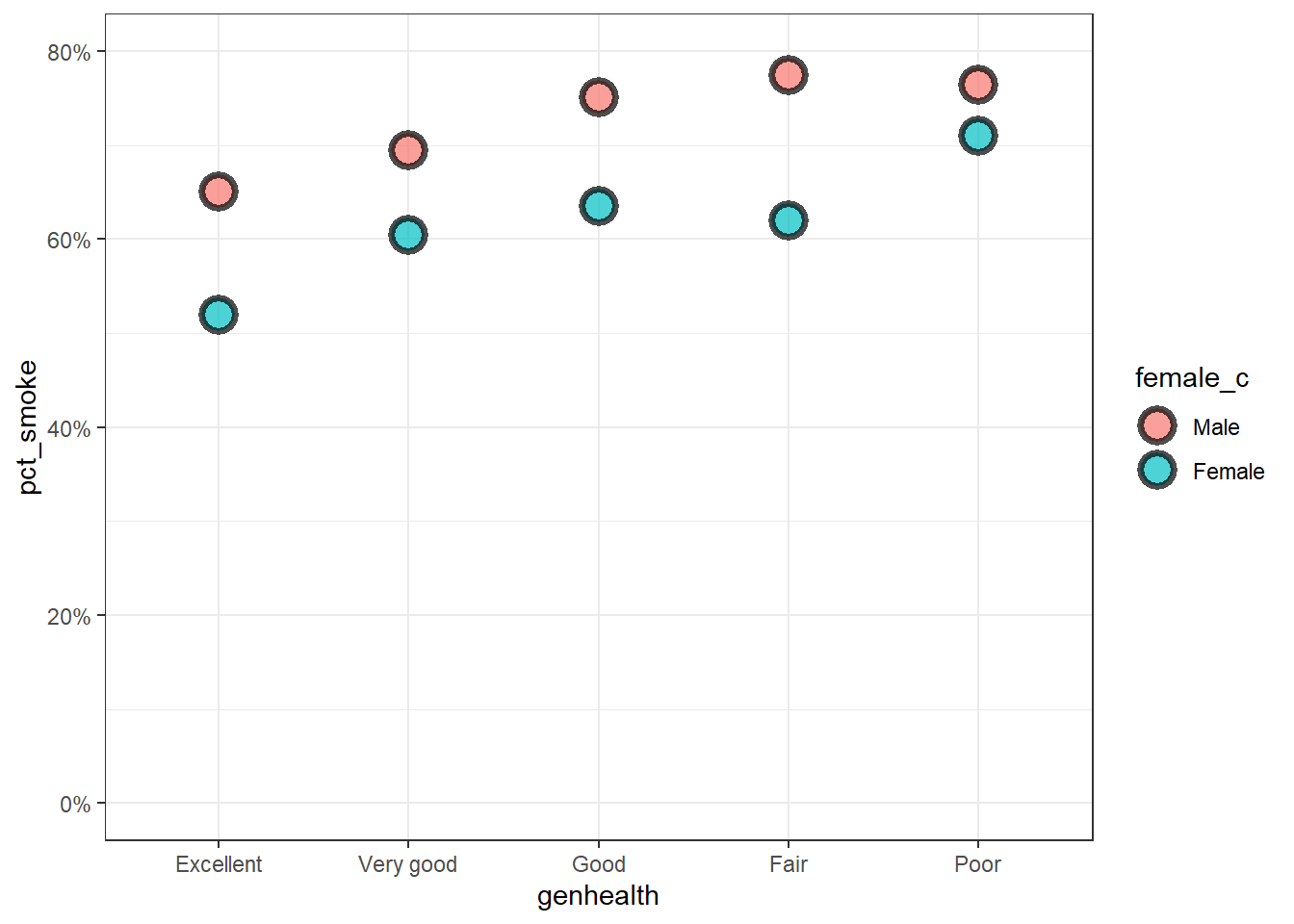
addhealth$female_c: Male

    Pearson's Chi-squared test

data:  x$eversmoke_c and x$genhealth
X-squared = 19.455, df = 4, p-value = 0.0006395

------------------------------------------------------------------------------------------------------------------------------------------------------ 
addhealth$female_c: Female

    Pearson's Chi-squared test

data:  x$eversmoke_c and x$genhealth
X-squared = 19.998, df = 4, p-value = 0.0004998

P-value still <.0001 in each group

The relationship between smoking status and general health is significant in both the main effects and the stratified model. The distribution of smoking status across general health categories does not differ between females and males. Gender is not a moderator for this analysis.

Example: Regression

ggscatter(iris, x="Sepal.Length", y = "Petal.Length", 
                     add = "reg.line", ellipse = TRUE)

Does the Species of an iris moderate the relationship between the length of the sepal and the length of it’s petal?

ggscatter(iris, x="Sepal.Length", y = "Petal.Length", add = "reg.line", 
          color = "Species", ellipse = TRUE)

The slope of the lowess line between virginica and versicolor appear similar in strength, whereas the slope of the line for setosa is closer to zero.

Example: Regression (cont.)

cor(iris$Sepal.Length, iris$Petal.Length)
[1] 0.8717538
by(iris, iris$Species, function(x) cor(x$Sepal.Length, x$Petal.Length))
iris$Species: setosa
[1] 0.2671758
------------------------------------------------------------------------------------------------------------------------------------------------------ 
iris$Species: versicolor
[1] 0.754049
------------------------------------------------------------------------------------------------------------------------------------------------------ 
iris$Species: virginica
[1] 0.8642247

\(r\) for virginica (.86) and veriscolor (.75) are similar to the overall correlation value (.87), but \(r\) for setosa (.27) is much smaller.

by(iris, iris$Species, function(x) {
  lm(x$Petal.Length ~ x$Sepal.Length) |> summary() |> broom::tidy()
  })
iris$Species: setosa
# A tibble: 2 × 5
  term           estimate std.error statistic p.value
  <chr>             <dbl>     <dbl>     <dbl>   <dbl>
1 (Intercept)       0.803    0.344       2.34  0.0238
2 x$Sepal.Length    0.132    0.0685      1.92  0.0607
------------------------------------------------------------------------------------------------------------------------------------------------------ 
iris$Species: versicolor
# A tibble: 2 × 5
  term           estimate std.error statistic  p.value
  <chr>             <dbl>     <dbl>     <dbl>    <dbl>
1 (Intercept)       0.185    0.514      0.360 7.20e- 1
2 x$Sepal.Length    0.686    0.0863     7.95  2.59e-10
------------------------------------------------------------------------------------------------------------------------------------------------------ 
iris$Species: virginica
# A tibble: 2 × 5
  term           estimate std.error statistic  p.value
  <chr>             <dbl>     <dbl>     <dbl>    <dbl>
1 (Intercept)       0.610    0.417       1.46 1.50e- 1
2 x$Sepal.Length    0.750    0.0630     11.9  6.30e-16

  • Overall: \(-7.1 + 1.86x\), p<.0001
  • Setosa: \(0.08 + 0.13x\), p=.06
  • Versicolor: \(0.19 + 0.69x\), p<.0001
  • Virginica: \(0.61 + 0.75x\), p<.0001

Iris specis moderates the relationship between sepal and petal length.