Simple Linear Regression

Robin Donatello

2023-10-23

Always visualized before you model

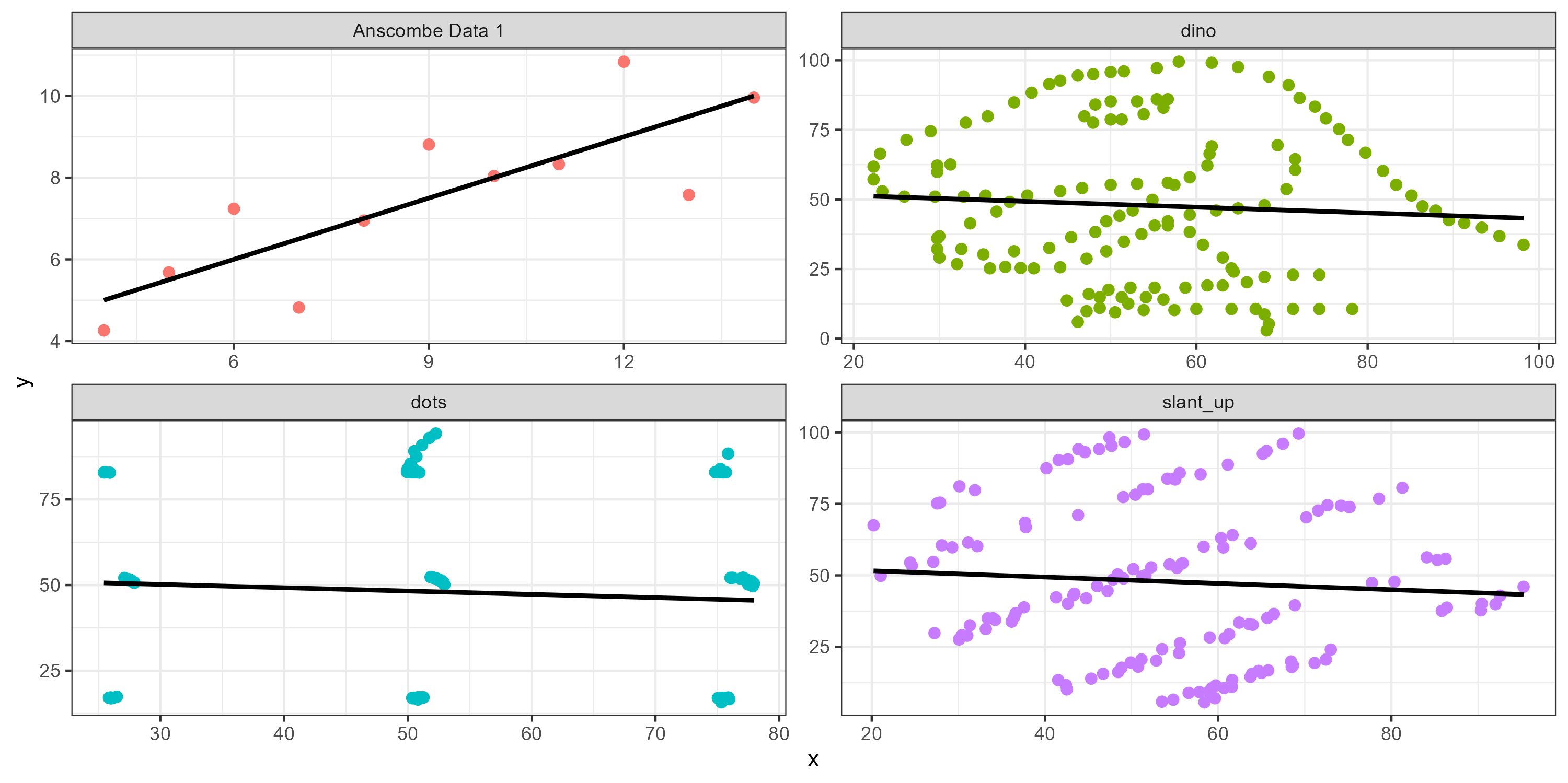
Anscombs Quartet are four datasets have the same correlation value and similar slope of the regression line.

So does this datasaurus!

Overview

The general purpose of regression is to learn more about the relationship between several independent or predictor variables and a quantitative dependent variable.

The goal of Simple linear regression is to describe the relationship between a continuous dependent variable Y and a single independent continuous variable X using a straight line.

External Instructional Notes

Applied Stats Course Notes

See ASCN Ch 7 for the learning content.

These slides contain an example of a full 5 step analysis.

Example: Body mass and bill length of penguins

1. Identify response and explanatory variables

  • The quantitative explanatory variable is body mass (g)
  • The quantitative response variable is bill length (mm)

2. Visualize and summarise bivariate relationship

Show the code
ggplot(pen, aes(x=body_mass_g, y=bill_length_mm)) + 
  geom_point() + geom_smooth(col = "red")

There is a strong, positive, mostly linear relationship between the body mass (g) of penguins and their bill length (mm) (r=.595).

3. Write the relationship you want to examine in the form of a research question.

  • Null Hypothesis: There is no linear relationship between body mass and bill length.
  • Alternate Hypothesis: There is a linear relationship between body mass and bill length.

4. Perform an appropriate statistical analysis using Dr D’s 4 step method.

a. Define parameters Let \(\beta_1\) be the true slope parameter that describes the change in bill length of the penguin as body mass increases.

b. State the null and alternative hypothesis as symbols

\(H_{0}: \beta_{1}=0 \qquad \qquad H_{A}: \beta_{1} \neq 0\)

c. State and justify the analysis model.

Both the outcome and predictor are continuous variables that have a visible linear relationship, and observations are independent.

The rest of the model assumptions can be checked after the model is fit using the check_model(my_model_object_name) function from the performance package.

d. Conduct the analysis and write a conclusion.

Show the code
pen.body.bill <- lm(bill_length_mm ~ body_mass_g, data=pen)
pen.body.bill |> summary()

Call:
lm(formula = bill_length_mm ~ body_mass_g, data = pen)

Residuals:
     Min       1Q   Median       3Q      Max 
-10.1251  -3.0434  -0.8089   2.0711  16.1109 

Coefficients:
             Estimate Std. Error t value Pr(>|t|)    
(Intercept) 2.690e+01  1.269e+00   21.19   <2e-16 ***
body_mass_g 4.051e-03  2.967e-04   13.65   <2e-16 ***
---
Signif. codes:  0 '***' 0.001 '**' 0.01 '*' 0.05 '.' 0.1 ' ' 1

Residual standard error: 4.394 on 340 degrees of freedom
  (2 observations deleted due to missingness)
Multiple R-squared:  0.3542,    Adjusted R-squared:  0.3523 
F-statistic: 186.4 on 1 and 340 DF,  p-value: < 2.2e-16

The p-value for \(b_{1}\) is <.0001, so there is sufficient evidence to believe that there is a linear relationship between body mass and bill length.

c (cont). Finish checking the assumptions

This section uses functions from the performance package.

Show the code
library(performance)

Assumption: Normality of residuals

Show the code
plot(check_normality(pen.body.bill))

The distribution of the residuals is mostly normal, pretty heavy right tail. This is indicative of a nonlinear trend somewhere in the data.

Assumption: Normality of residuals

Show the code
plot(check_normality(pen.body.bill), type = "qq")

This is also known as a ‘normal probability plot’ or a ‘qqplot’. It is used to compare the theoretical quantiles of the data if it were to come from a normal distribution to the observed quantiles. PMA6 Figure 5.4 has more examples and an explanation.

Assumption: Homogeneity of variance

Show the code
plot(check_heteroskedasticity(pen.body.bill))

Holy non-flat relationship Batman. The variance of Y is not constant. This is a warning that our linear model does not fit the data well and we should look into possible refinements and improvements.

Model-check Posterior Predictions

Show the code
plot(check_posterior_predictions(pen.body.bill))

This check compares the distribution of predicted values to the distribution of observed values. In this example the observed distribution of bill length is bimodal, and so the model is overestimating some values and underestimating others. There is clearly some other confounding variable that predicts bill length better than just body mass.

5. Write a conclusion in context of the problem.

Show the code
pen.body.bill |> coefficients() 
 (Intercept)  body_mass_g 
26.898872424  0.004051417 
Show the code
pen.body.bill |> confint()
                   2.5 %       97.5 %
(Intercept) 24.402502194 29.395242653
body_mass_g  0.003467795  0.004635038
Show the code
pen.body.bill |> r2()
# R2 for Linear Regression
       R2: 0.354
  adj. R2: 0.352

Each 1g increase in body mass of a penguin is associated with a significant increase of 0.004 (0.0035, 0.0046) mm of bill length (p<.0001).

An increase of 1kg of body mass in a penguin corresponds to a 4(3.5, 4.6) mm increase in bill length.

Body mass explains 35.4% of the variation in bill length.

However, model diagnostics indicate that a linear model may not be appropriate for this relationship. The assumption of constant variance is not upheld and there may be another variable that affects bill length.