Show the code
2025-10-13
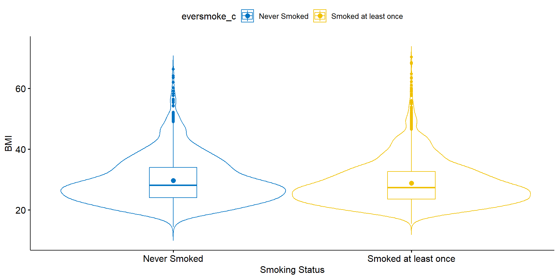
Smokers have on average BMI of 28.8, smaller than the average BMI of non-smokers at 29.7. Non-smokers have more variation in their weights (7.8 vs 7.3lbs), but the distributions both look normal, if slightly skewed right.
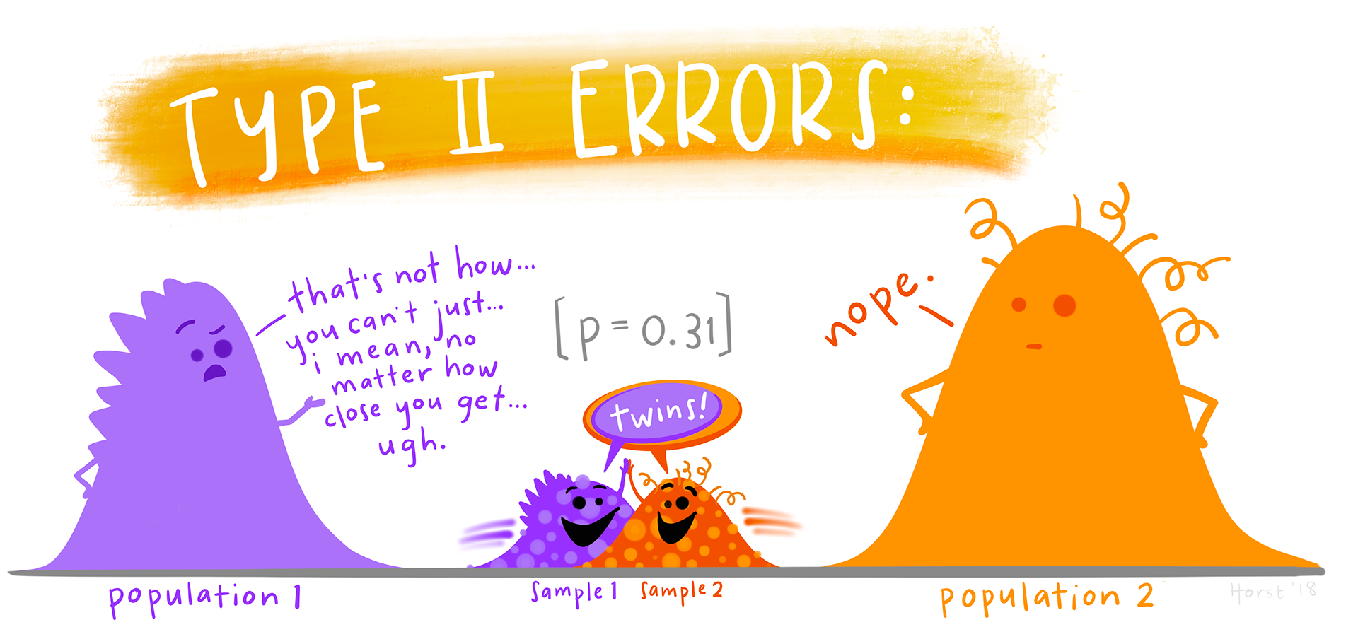
Samples come from the same population (\(\mu_1 - \mu_2\))
Credit: Allison Horst https://allisonhorst.com/
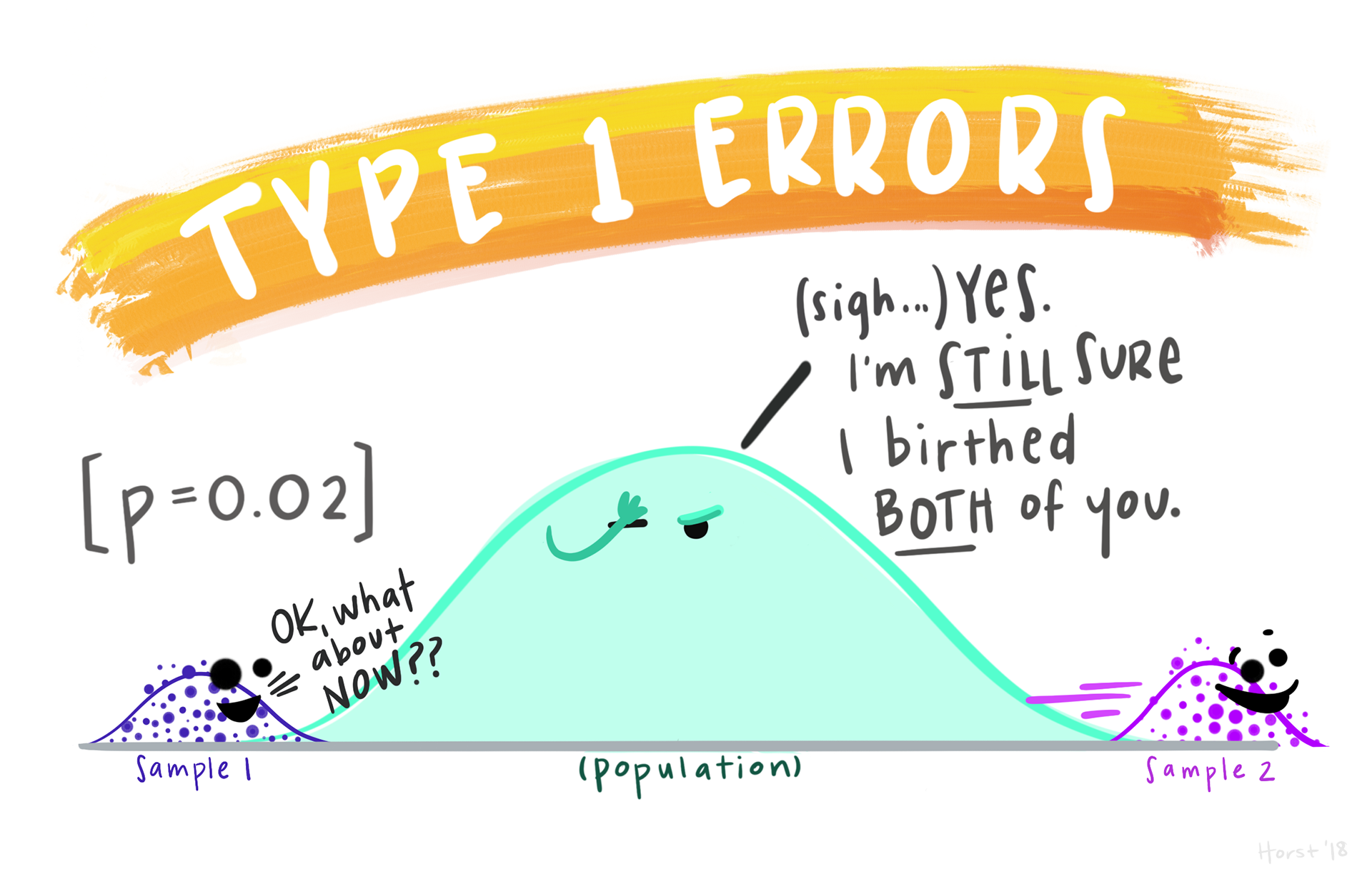
Credit: Allison Horst https://allisonhorst.com/
Credit: Allison Horst https://allisonhorst.com/