Simple Linear Regression Modeling

Robin Donatello

2024-10-28

Purpose & Estimation

Purpose of Regression Modeling

  • Learn more about the relationship between several independent or predictor variables and a quantitative dependent (response) variable.
  • Regression is widely used in research as it allows us to ask the general question “what is the best predictor of…”, and does “additional variable A” or “additional variable B confound the relationship between my explanatory and response variable?

Both Regression and Correlation can be used to

  • Descriptive: Draw inferences regarding the relationship
  • Predictive: Predict the value of \(Y\) for given values of one or more \(X\)’s.

Examples in practice

  • Educational researchers might want to learn about the best predictors of success in high-school.
  • Sociologists may want to find out which of the multiple social indicators best predict whether or not a new immigrant group will adapt to their new country of residence.
  • Biologists may want to find out which factors (i.e. temperature, barometric pressure, humidity, etc.) best predict caterpillar reproduction.

Example - Lung function

Lung function data were obtained from an epidemiological study of households living in four areas with different amounts and types of air pollution. The data set used in PMA6 is a subset of the total data. In this example we use only the data taken on the fathers, all of whom are nonsmokers.

One of the major early indicators of reduced respiratory function is FEV1 or forced expiratory volume in the first second (amount of air exhaled in 1 second). Since it is known that taller males tend to have higher FEV1, we wish to determine the relationship between height and FEV1. We can use regression analysis for both a descriptive and predictive purpose.

  • Descriptive: Describing the relationship between FEV1 and height
  • Predictive: Determine the expected or normal FEV1 for a given height

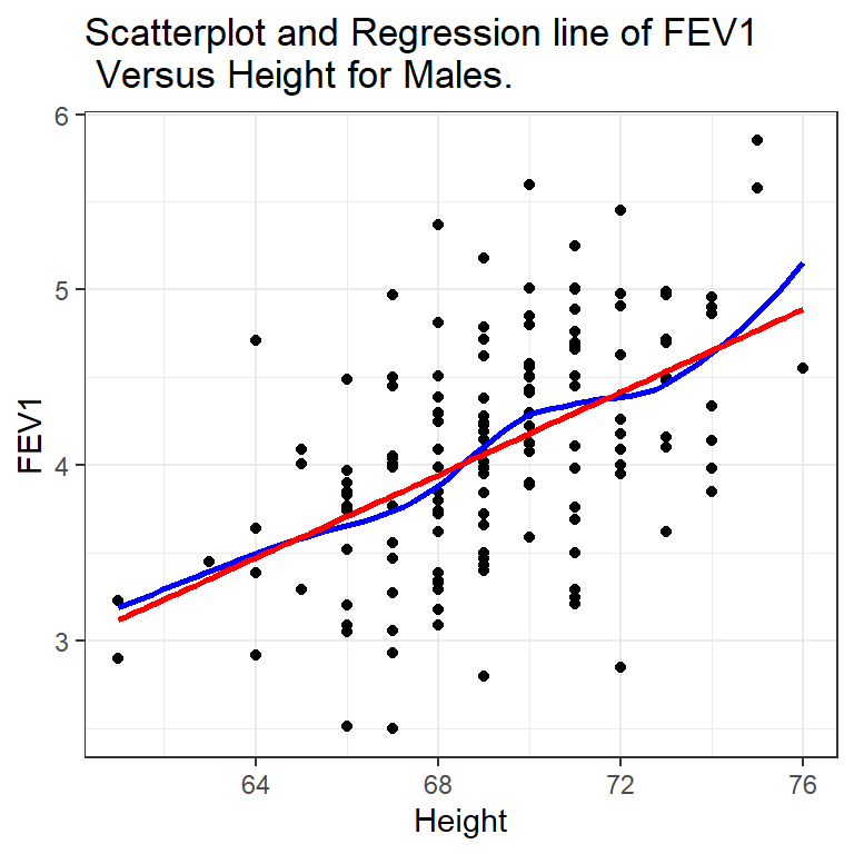
Visualize the relationship

Show the code
ggplot(fev, aes(y=FFEV1, x=FHEIGHT)) + 
  geom_point() + geom_smooth(se=FALSE, col="blue") + 
  geom_smooth(se=FALSE, method = "lm", col="red") + 
      xlab("Height") + ylab("FEV1") + 
      ggtitle("Scatterplot and Regression line of FEV1 \n Versus Height for Males.") + theme_bw() 


There does appear to be a tendency for taller men to have higher FEV1. Since this relationship is reasonably linear (the blue loess line is similar to the red linear line) we can write the model the population average FEV \(\mu_{y}\) as a linear function of height \(x\):

\[ \mu_{y} = \beta_{0} + \beta_{1}x \]

The intercept parameter, \(\beta_{0}\), represents where the line crosses the y-axis when \(x=0\). The slope parameter, \(\beta_{1}\), represents the change in \(\mu_{y}\) per 1 unit \(x\).

Unifying model framework

We know that there is always random noise in real data (DATA = MODEL FIT + RESIDUAL) so we introduce a random error term, \(\epsilon_{i}\) and assume the model:

\[ y_{i} = \beta_{0} + \beta_{1} X + \epsilon_{i} \\ \epsilon_{i} \sim N(0, \sigma^{2}) \]

This model states that the random variable \(y\) to be made up of a predictable part (a linear function of \(x\)) and an unpredictable part (the random error, \(\epsilon_{i}\)). The error (residual) term includes the effects of all other factors, known or unknown.

Least Squares Estimation

  • Most common method of fitting a straight line to two variables.
  • Also known as “Ordinary Least Squares (OLS)”
  • Calculates sample statistics \(b_{0}\) and \(b_{1}\) to estimate the population parameter values \(\beta_{0}\) and \(\beta_{1}\)
  • The estimated mean function is \(\hat{y}_{i} = b_{0} + b_{1}x_{i}\)
  • The fitted value, \(\hat{y}_{i}\), is the estimated value for point \(i\), calculated by plugging in a value for \(x_{i}\) and calculating the result.
  • The residual is the difference between the observed and the fitted value: \(\epsilon_{i} = y_{i}-\hat{y}_{i}\)

Least Squares Estimation

The estimates \(b_{0}\) and \(b_{1}\) are found such that they minimize the sum of the squared residuals (the unexplained residual error)

\[ \sum_{i=1}^{n} \epsilon_{i} \]

For simple linear regression the regression coefficient estimates that minimize the sum of squared errors can be calculated as:

\[ \hat{\beta_{0}} = \bar{y} - \hat{\beta_{1}}\bar{x} \quad \mbox{ and } \quad \hat{\beta_{1}} = r\frac{s_{y}}{s_{x}} \]

where \(r\) is the correlation coefficient between \(x\) and \(y\).

Partitioning the Variance

Revisiting the Sum of Squares

Go to: https://paternogbc.shinyapps.io/SS_regression/. Then turn and talk to your group about the following features of the Sum of Squares Graphs

Total

  • What are the dots?
  • What does the horizontal line represent?
  • What do the blue lines represent?

Regression

  • What does the horizontal line represent?
  • What does the sloped line represent?
  • What are the green lines?

Error

  • What are the dots?
  • What does the sloped line represent?
  • What do the red lines represent?

Sum of Squares - Regression

  • SS Total- how far are the points away from \(\bar{y}\)?
  • SS Regression - how far away is the regression line from \(\bar{y}\)?
  • SS Error - how far are the points away from the estimated regression line?

Looking at it this way, we are asking “If I know the value of \(x\), how much better will I be at predicting \(y\) than if I were just to use \(\bar{y}\)?

Fitting the model

Least Squares Estimation - in R

A linear model using least squares estimation can be performed in R using the function lm(y ~ x)

fev.model <- lm(FFEV1 ~ FHEIGHT, data = fev)
fev.model

Call:
lm(formula = FFEV1 ~ FHEIGHT, data = fev)

Coefficients:
(Intercept)      FHEIGHT  
    -4.0867       0.1181  

The regression equation for the model to explain FEV1 using height as a predictor is:
\[ \hat{y} = -4.087 + 0.118x \]

Using this model

\[ \hat{y} = -4.087 + 0.118x \]

  • \(b_{0}\): For a father that is 0 cm tall, the predicted FEV is -4.087 (an impossible result)
  • \(b_{1}\): For every additional cm taller a father is, his predicted FEV increases by 0.118L.
  • \(\hat{y}_{x=70}\): A father who is 70cm tall has a predicted FEV1 of \(-4.087 + 0.118(70) = 4.17L\)

Other facts about LS regression

  • A change of one sd in \(x\) corresponds to a change of \(r\) sd in \(y\) since \(b_{1}=r\frac{s_{y}}{s_{x}}\).
  • If the correlation is 0, the slope of the LS line is 0. A test of \(\beta_{1}=0\) is equivalent to a test of \(\rho=0\).
  • The LS line always passes through the point \((\bar{x}, \bar{y})\).
  • The distinction between explanatory and response variables is essential in regression. Reversing \(x\) and \(y\) results in a different regression line.
  • The Root Mean Squared Error (RMSE) is an estimate for \(\sigma\).

Assumptions

Mathematical Model

The mathematical model that we use for regression has these features that translate into assumptions.

\[ \begin{align} Y|X & \sim N(\mu_{Y|X}, \sigma^{2}) \\ \mu_{Y|X} & = \beta_{0} + \beta_{1} X \\ \sigma^{2} & = Var(Y|X) \end{align} \]
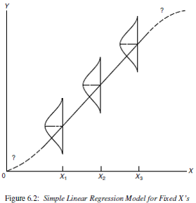
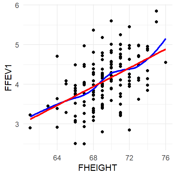
Figure 6.2
  • Independence The observations are the result of a simple random sample and thus are independent from each other
  • Linearity: The mean of \(Y\) values at any given \(X\) follows a straight line
  • Normality: \(Y\) values are normally distributed at any given \(X\)
  • Homoscedasticity The variance of \(Y\) values at any \(X\) is \(\sigma^2\) (same for all X)
  • The last two assumptions are checked by examining the residuals, and so can only be checked after the model has been fit.

Assumption - Independence

  • Knowledge of the method of data collection here is key!
  • If the sampling method is not random, observations may not be independent.
  • No real good way to “test” for independence. Need to know how the sample was obtained.
  • Non simple random sample will not result in the same variance estimates
  • Can use hierarchical/multi-level models for clustered samples

Assumption - Linearity

  • Slight departures OK
  • Can use transformations of strongly skewed data to achieve it
  • The lowess trend line reasonably follows a linear pattern.
ggplot(fev, aes(y=FFEV1, x=FHEIGHT)) + 
  geom_point() + 
  geom_smooth(col="blue", se=FALSE) + 
  geom_smooth(method = "lm", col="red", se=FALSE)

Assumption - Normality

  • Slight departures OK
  • Can use transformations to achieve it

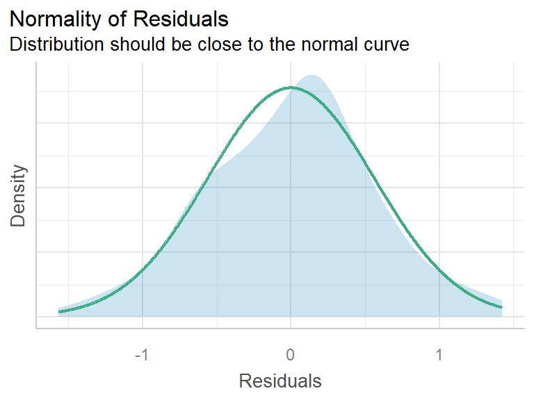
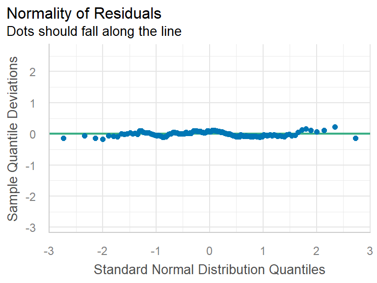
These plots are generated from the performance package.

plot(check_normality(fev.model), type="density")
plot(check_normality(fev.model), type="qq")
  • The residuals follow a normal distribution well.
  • Don’t let the pattern of the residuals on the qqplot fool you, the y-axis is very zoomed in.

Assumption - Homoscedasticity

Show the code
plot(check_heteroskedasticity(fev.model))

  • If the variance (std. residual) changes with the value of \(\hat{y}\), that is a sign of non-constant variance.
  • Violations result in reduced validity of inference and typically larger standard errors for the coefficients.
  • Could be caused by outliers or model mis-specificiation (e.g. non-normal data)
  • FEV Example - even though there is a slight increase in the trend of fitted values against the residuals, this is within the tolerance range.

Out of range predictions


Figure 6.2

Caution!

The linear model is only valid within the range of the data used to fit the model

To take an extreme example, suppose a father was 2 feet tall. Then the equation would predict an impossible negative value of FEV1 (\(-1.255\)).

A safe policy is to restrict the use of the equation to the range of the \(X\) observed in the sample.

Model-check

Show the code
plot(check_posterior_predictions(fev.model))

Another way of assessing model fit is to check the distribution of the predictions created by this model. A good fitting model should predict values that are similar to the observed data used to fit the model.

Inference

Distribution of parameter estimates

  • The estimated coefficients are functions of both \(x\) and \(y\), and they are not themselves independent of each other (e.g. \(Cov(b_{0}, b_{1}) \neq 0)\).
  • The joint vector \(\hat{\beta}(y, x)= (b_{0}, b_{1})\) has a multivariate normal distribution, with variance that depends on the predictor variables \(x\) only.

\[ \hat{\beta}(y, x) \sim \mathcal{N}(\beta, \mathbf{x^{T}x}^{-1}\sigma^{2}) \]

  • The normality of the vector \(\hat{\beta}\) is quite robust to the model assumptions.
  • Even if the residuals are not normally distributed, the CLT ensures that the \(\hat{\beta}\) are close to normal
  • When sample sizes are low in a category, or \(Var(X)\) is close to zero, \(x^{T}x\) can’t be inverted - leading to errors of “non positive definite”

Calculating Confidence Intervals

\[ b_{p} \pm 1.96*SE(b_{p})\]

point estimate \(\pm\) critical value * standard error of estimate

But calculating the variance of \(b_{p}\) involves \(\mathbf{x^{T}x}^{-1}\sigma^{2}\), which is outside the scope of this class. So, we use R functions

confint(fev.model)
                  2.5 %     97.5 %
(Intercept) -6.36315502 -1.8102499
FHEIGHT      0.08526328  0.1509472

We can be 95% confident that the true slope parameter between a fathers height and his FEV1 is contained in the interval (0.085, 0.151).

Hypotheis Testing

Let \(\beta_1\) be the true slope parameter that describes the change in FEV1 as a function of height in cm.

  • \(H_{0}: \beta_{1}=0\) There is no linear relationship between FEV1 and Height
  • \(H_{A}: \beta_{1} \neq 0\) Alternate Hypothesis: There is a linear relationship between FEV1 and Height
Show the code
broom::tidy(fev.model) |> kable(digits=3) #kable is in the knitr package
term estimate std.error statistic p.value
(Intercept) -4.087 1.152 -3.548 0.001
FHEIGHT 0.118 0.017 7.106 0.000

The p-value for \(b_{1}\) is <.0001, so there is sufficient evidence to believe that there is a linear relationship between FEV1 and Height of fathers.

Write a conclusion

Base R (ish)

fev.model |> coefficients() 
(Intercept)     FHEIGHT 
 -4.0867025   0.1181052 
fev.model |> confint()
                  2.5 %     97.5 %
(Intercept) -6.36315502 -1.8102499
FHEIGHT      0.08526328  0.1509472
fev.model |> r2() # from the performance package
# R2 for Linear Regression
       R2: 0.254
  adj. R2: 0.249

gtsummary package

tbl_regression(fev.model) %>% 
  add_glance_table(include = c(nobs, r.squared))
Characteristic Beta 95% CI1 p-value
FHEIGHT 0.12 0.09, 0.15 <0.001
No. Obs. 150
0.254
1 CI = Confidence Interval

Conclusion

Each 1cm increase in height of a father is associated with a significant increase of 0.118 (0.09, 0.15) L of FEV1 (p<.0001). Height explains 25.4% of the variation in FEV1.