Correlation Analysis

Robin Donatello

2024-10-23

Opening Remarks

The PMA6 textbook (Chapter 7) goes into great detail on this topic, since regression is typically the basis for all advanced models.

The book also distinguishes between a “fixed-x” case, where the values of the explanatory variable \(x\) only take on pre-specified values, and a “variable-x” case, where the values of \(x\) are observations from a population distribution of X’s.

This latter case is what we will be concerning ourselves with.

Bivariate distribution

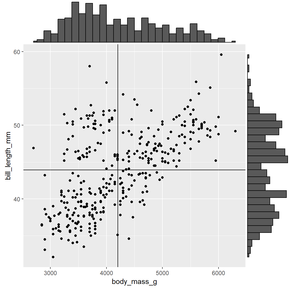
The bivariate distribution describes how of \(X\) and \(Y\) are jointly distributed, and is best interpreted by a look at the scatter diagram.

Show the code

y.bar <- mean(pen$bill_length_mm, na.rm=TRUE)
x.bar <- mean(pen$body_mass_g, na.rm=TRUE)

p <- ggplot(pen, aes(x=body_mass_g, y=bill_length_mm)) + geom_point() + 
  geom_hline(yintercept = y.bar) + 
  geom_vline(xintercept = x.bar) 
ggExtra::ggMarginal(p, type="histogram")

If \(X\) and \(Y\) come from independent normal distributions, the pair \((X,Y)\) comes from a bivariate normal distribution, and the data will tend to cluster around the means of \(X\) and \(Y\).

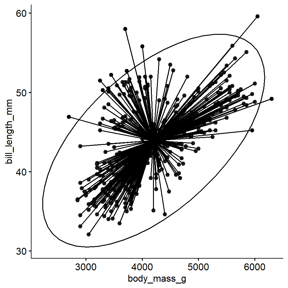
Ellipse of concentration

We can view the ellipse of concentration as measure of strength and direction of the correlation between X and Y.

Show the code

ggpubr::ggscatter(pen, x = "body_mass_g", y = "bill_length_mm",
   ellipse = TRUE, mean.point = TRUE,
   star.plot = TRUE)

See PMA6 Figure 7.5 for more examples.

Correlation

The correlation coefficient is designated by \(r\) for the sample correlation, and \(\rho\) for the population correlation. The correlation is a measure of the strength and direction of a linear relationship between two variables.

The correlation ranges from +1 to -1. A correlation of +1 means that there is a perfect, positive linear relationship between the two variables. A correlation of -1 means there is a perfect, negative linear relationship between the two variables. In both cases, knowing the value of one variable, you can perfectly predict the value of the second.

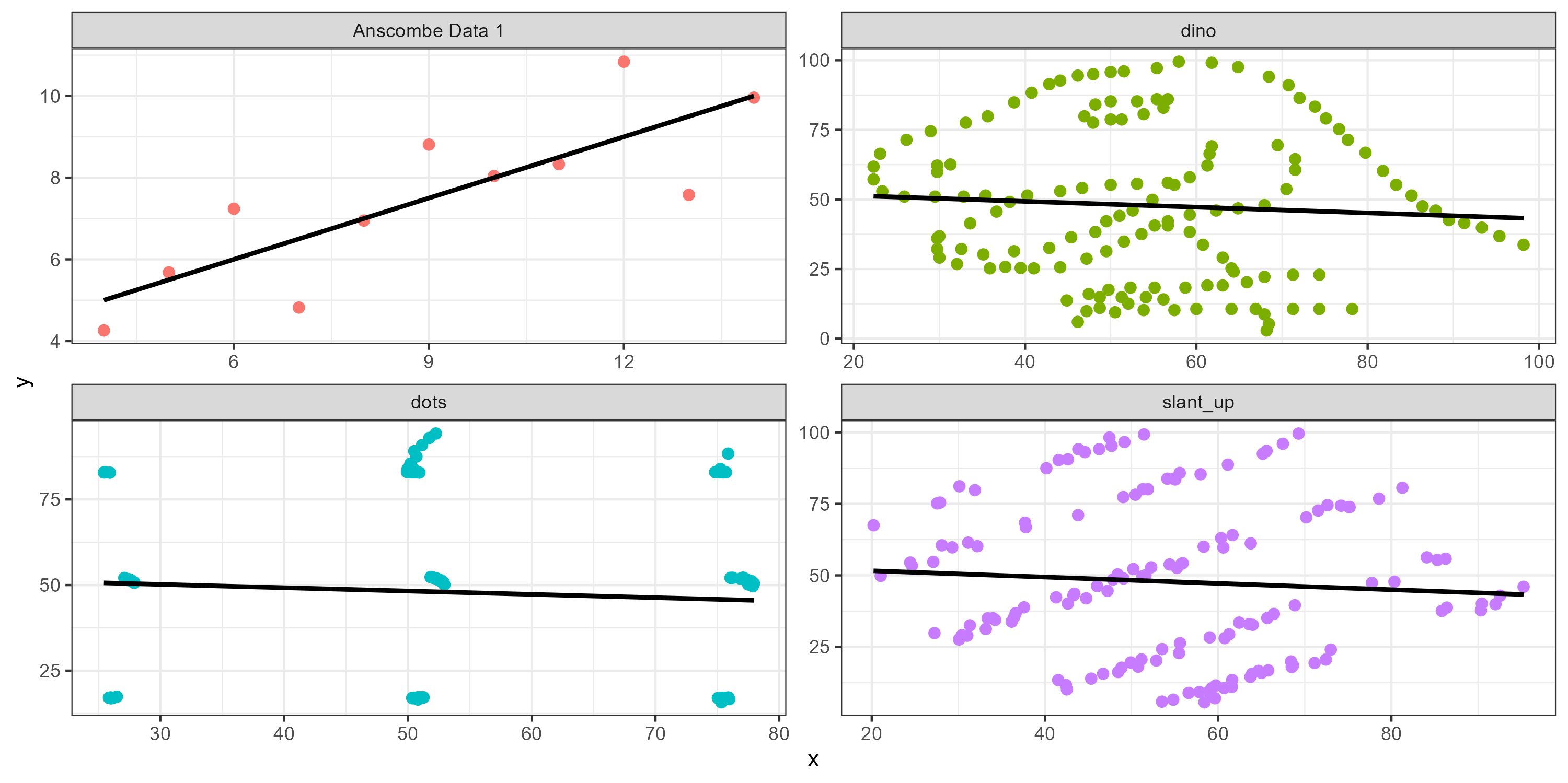
Reminder to visualize your data before analysis

These all have the same r value

Strength of the correlation

Here are rough estimates for interpreting the strengths of correlations based on the magnitude of \(r\).

\(|r| \geq 0.7\): Very strong relationship
\(0.4 \leq |r| < 0.7\): Strong relationship
\(0.3 \leq |r| < 0.4\): Moderate relationship
\(0.2 \leq |r| < 0.3:\) Weak relationship
\(|r| < 0.2:\) Negligible or no relationship

As a measure of model fit

When we square \(r\) (i.e. \(R^{2}\)), it tells us what proportion of the variability in one variable that is described by variation in the second variable.

Yes, this is mathematically the same as the coefficient of determination we saw in ANOVA.

Pearson test of correlation

To test for a linear correlation between two variables we use the Pearson correlation coefficient which is defined as the covariance of the two variables divided by the product of their standard deviations.

\[ \rho_{X,Y} = \frac{cov(X,Y)}{\sigma_{x}\sigma_{Y}} \]

There are many modifications and adjustments to this measure that we will not get into detail with. We are using correlation as a stepping stool to Linear Regression.

Example: Body mass and bill length of penguins

1. Identify response and explanatory variables

The quantitative explanatory variable is body mass (g)
The quantitative response variable is bill length (mm)

2. Visualize and summarise

Show the code

ggplot(pen, aes(x=body_mass_g, y=bill_length_mm)) + 
  geom_point() + geom_smooth(col = "red")

Show the code

cor(pen$body_mass_g, pen$bill_length_mm, use = "pairwise.complete.obs")

[1] 0.5951098

There is a strong, positive, mostly linear relationship between the body mass (g) of penguins and their bill length (mm) (r=.595).

3. Write the null and research hypothesis in words and symbols.

Null Hypothesis: There is no correlation between the body mass and bill length of penguins.
Alternate Hypothesis: There is a correlation between the body mass and bill length of penguins.

Let \(\rho\) be the true correlation between body mass and bill length of penguins.

\(H_{0}: \rho=0 \qquad \qquad H_{A}: \rho \neq 0\)

4. State and justify the analysis model. Check assumptions.

Pearsons test of correlation will be conducted. This is appropriate because both variables are quantitative.
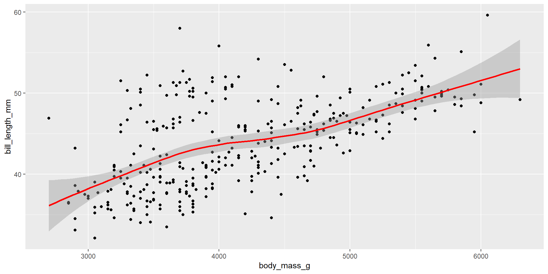
The relationship between variables are reasonably linear
The sample size is large.

5. Conduct the test

And make a decision about the plausibility of the alternative hypothesis.

Show the code

cor.test(pen$body_mass_g, pen$bill_length_mm)


    Pearson's product-moment correlation

data:  pen$body_mass_g and pen$bill_length_mm
t = 13.654, df = 340, p-value < 2.2e-16
alternative hypothesis: true correlation is not equal to 0
95 percent confidence interval:
 0.5220040 0.6595358
sample estimates:
      cor 
0.5951098

The p-value is very small, there is evidence in favor of a non-zero correlation.

6. Write a conclusion in context of the problem.

There was a statistically significant and strong correlation between the body mass (g) and bill length (mm) of penguins (r = 0.595, 95%CI .5220-.6595, p < .0001). The significant positive correlation shows that as the body mass of a penguin increases so does the bill length. These results suggest that 35% (95% CI: 27.2-43.5) of the variance in bill length can be explained by the body mass of the penguin.