Statistical Inference using Models
Robin Donatello
2025-10-06
Warm up exercise
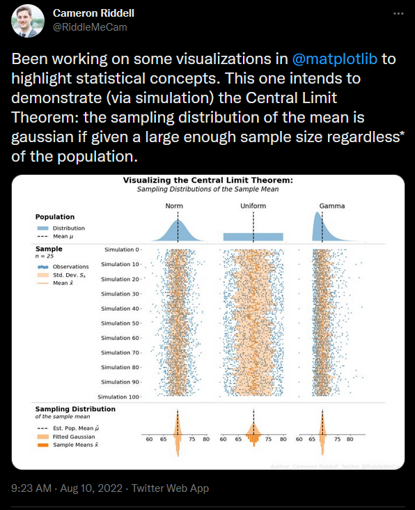
Work through the Central Limit Theorem interactive explorer for about 15 minutes. Follow the instructions on the app and take notes and be prepared to share out what you learned/your take away message.
Sampling Distributions
Since point estimates are numbers calculated on a sample, they are also sample statistics. Recall that sample statistics are used to estimate parameters, the true value of the quantity of interest from the population.
As we just saw through simulation, point estimates are subject to random variation because they are calculated on different random samples from the population. The distribution of repeatedly calculated point estimates based on the same fixed size \(n\) from a population is called a sampling distribution.
Mathematical theory guarantees
- If repeated samples are taken, a point estimate will follow something that resembles a normal distribution when certain conditions are met.
- Note: we typically only take one sample, but the mathematical model lets us know what to expect if we had taken repeated samples
Observations in the sample are independent.
Guaranteed when we take a random sample from a population, or randomly divide individuals into treatment and control groups.
The sample is large enough.
What qualifies as “large enough” differs from one context to the next. If the population is already normally distributed and the formula to calculate the sample statistic simple, then fewer samples are needed. The “magic” number 30 gets thrown around a lot.
The Normal Distribution
The normal distribution is used to describe the variability associated with sample statistics which are taken from either repeated samples or repeated experiments. The normal distribution is quite powerful in that it describes the variability of many different statistics such as the sample mean and sample proportions.
Distributions of many variables are nearly normal, but none are exactly normal. While not perfect for any single problem, the Normal Distribution is very useful for a variety of problems.
The Normal Distribution
Pre-requisite knowledge
It is expected that you have a basic understanding of the Normal distribution. If you need a detailed refresher, refer to IMS 13.2.
What follows is a quick recap of critical details.
Distributional Notation
\[ X \sim \mathcal{N}(\mu, \sigma^2)\] This means some random variable \(X\) is distributed(\(\sim\)), as a Normal (\(\mathcal{N}\)) distribution centered on mean \(\mu\) with variance \(\sigma^{2}\).
Notational differences
Note that the IMS textbook uses the uncommon notation \(\mathcal{N}(\mu, \sigma)\), where the second parameter is \(\sigma\), the standard deviation.
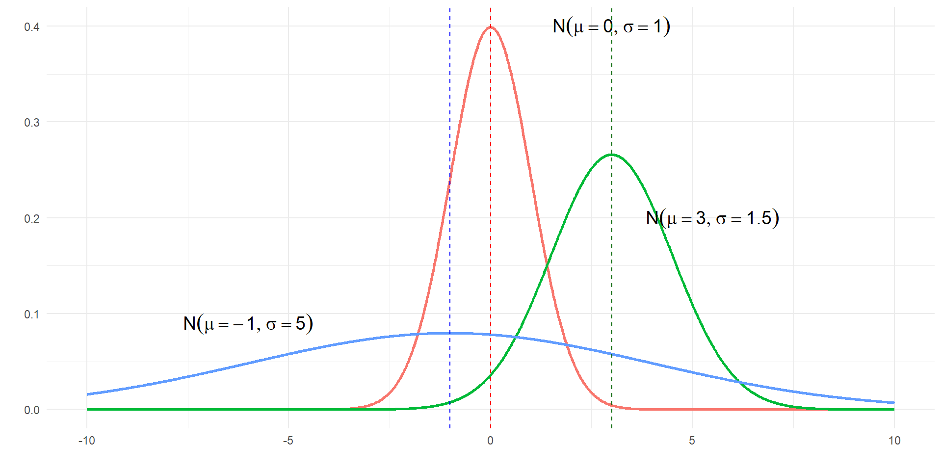
The Normal Distribution
- Symmetric, “bell shaped”
- Centered on \(\mu\) and spread controlled by \(\sigma^2\)
- Tails extend to \(\infty\)
- Area under the curve will always add to 1.
- Used to calculate the probability of an event occurring
Comparing values under two different distributions
Two different college-ready exams
SAT scores follow a nearly normal distribution with a mean of 1500 points and a standard deviation of 300 points.
ACT scores also follow a nearly normal distribution with mean of 21 points and a standard deviation of 5 points.
Suppose Nel scored 1800 points on their SAT and Sian scored 24 points on their ACT.
Who performed better?
Standardizing Distributions
If you overlay the two distributions, where the means line up and where each tick mark represents one standard deviation away from the mean, we can see who did better relative to the exam average.
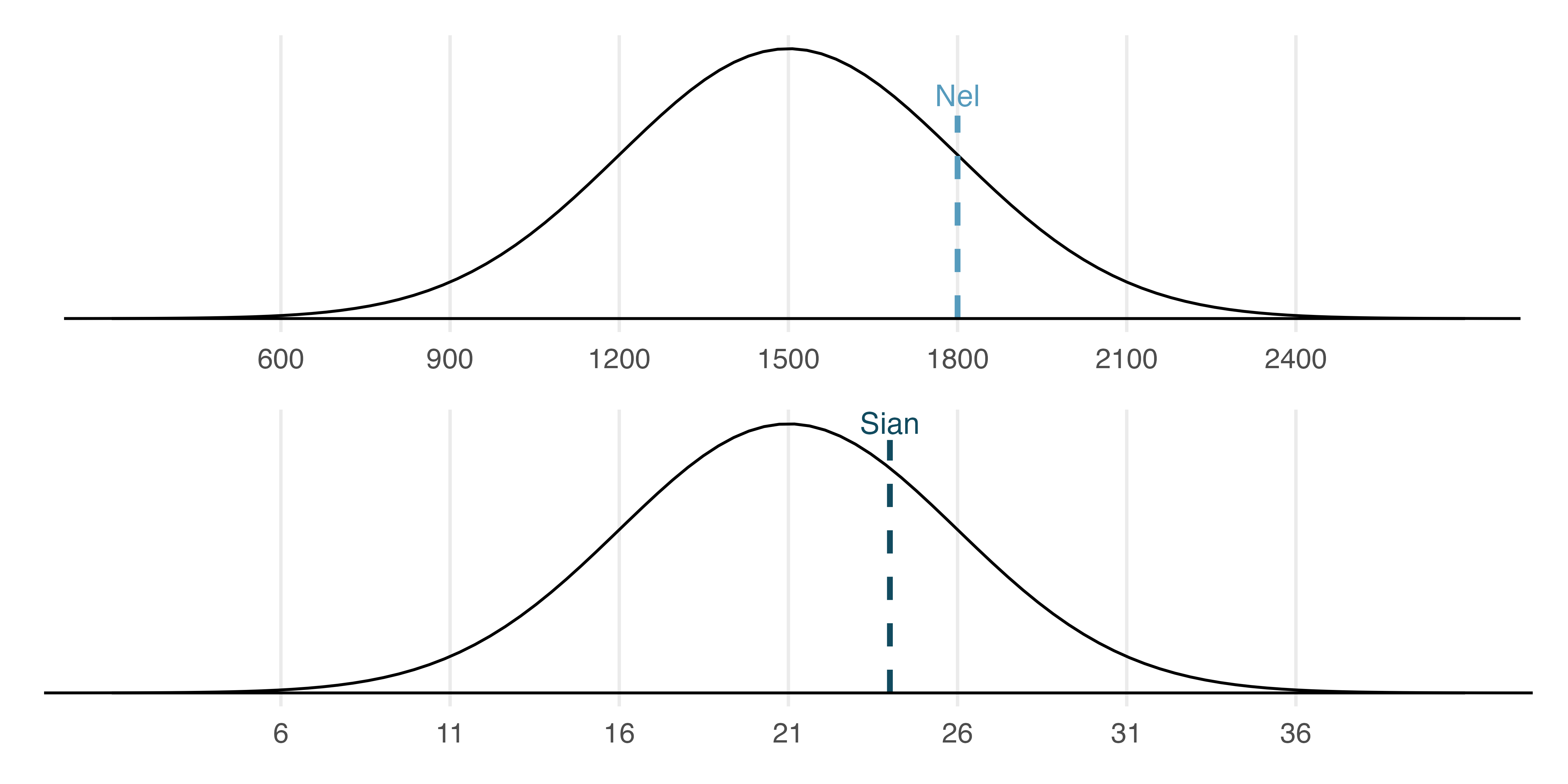
\[X_{SAT} \sim \mathcal{N}(1500, 300^{2})\]
\[X_{ACT} \sim \mathcal{N}(21, 25)\]
Z-score
The Z score of an observation is the number of standard deviations it falls above or below the mean. We compute the Z score for an observation that follows a distribution with mean and standard deviation using
\[ Z = \frac{x- \mu}{\sigma} \] If an observation \(x\) comes from a \(\mathcal{N}(\mu, \sigma)\) distribution, then \(Z \sim \mathcal{N}(0, 1)\). We center the distribution by subtracting the mean, and scale by dividing by the sd.
Comparing Scores
Calculate the Z-score for both Nel and Sian. Who did better?
- \(X_{SAT} \sim \mathcal{N}(1500, 300^{2})\)
- \(x_{Nel} = 1800\)
- \(Z_{Nel} = \frac{1800- 1500}{300} = 1\)
- \(X_{ACT} \sim \mathcal{N}(21, 25)\)
- \(x_{Sian} = 24\)
- \(Z_{Sian} = \frac{24- 21}{5} = 0.6\)
Comparing Scores
While we know Nel did better, Sian didn’t do too bad! What was their percentile (The percent of observations below a specified value)?
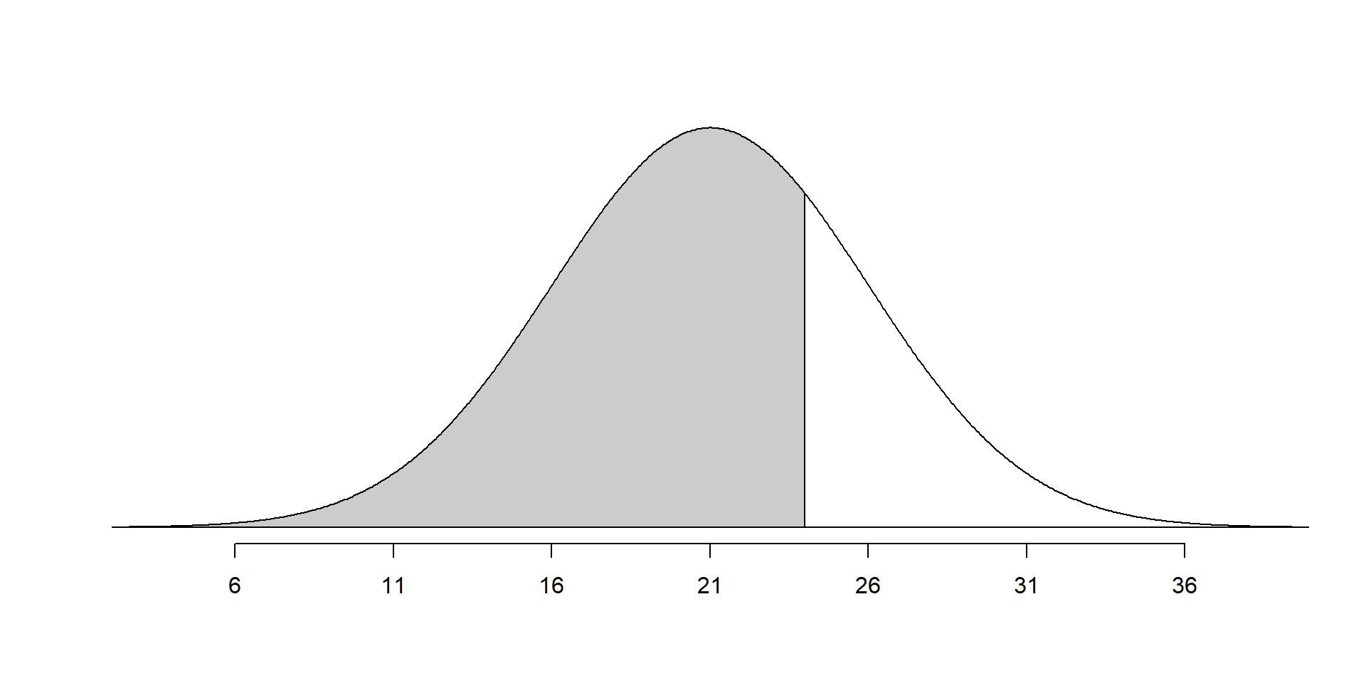
Finding percentiles
If \(X \sim \mathcal{N}(\mu, \sigma^{2})\), then pnorm calculates the probability that a value is below a certain number a.
- \(P(X < a)\) is found using
pnorm(a, mean, sd)
A complementary function, qnorm calculates the cutoff value a that is needed such that a certain percent of observations (q) are below that value.
- \(P(X < a) = q\) is found using
qnorm(q, mean, sd)
You would need to score a 27.5 to be in the top 10th percentile of ACT test takers.
Quantifying variability of a statistic
Follows IMS 13.3
Many estimates are normally distributed
- the sample proportion \(\hat{p}\)
- the sample mean \(\bar{x}\)
- differences in two sample proportions \(\hat{p}_{1} - \hat{p}_{2}\)
- differences in two sample means \(\bar{x}_{1} - \bar{x}_{2}\)
- the sample slope from a linear model \(\hat{\beta}\)
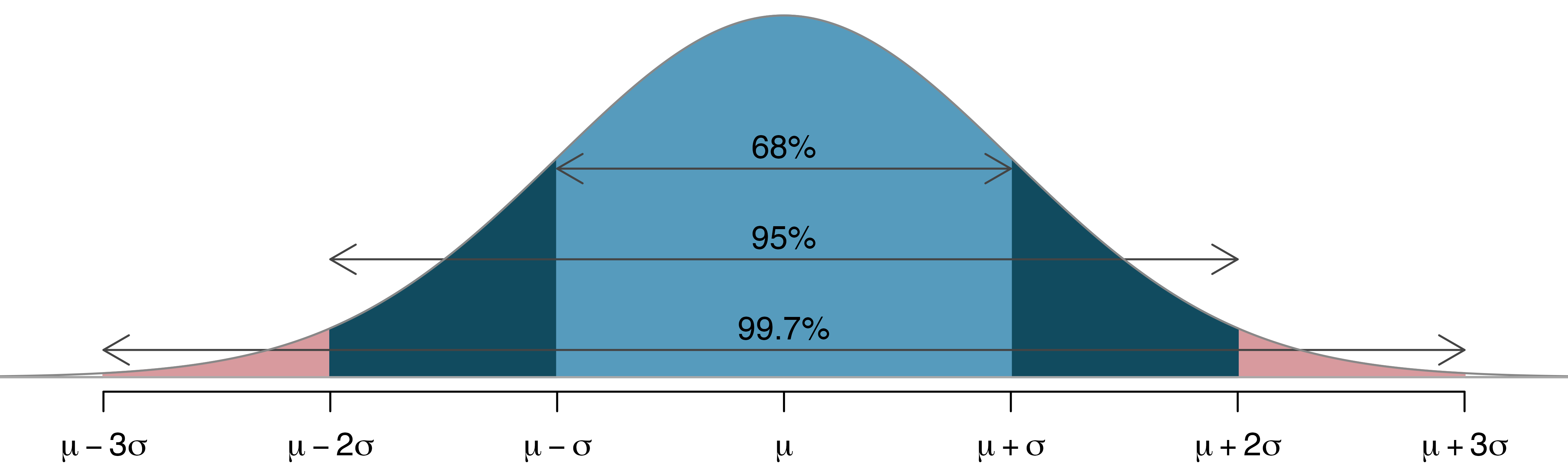
68-95-99.7 rule of thumb
Because intuition is important.
SD vs SE
Definition: Standard Deviation (SD)
Variability of the data values (\(x\))
Definition: Standard Error (SE)
Variability of the sample statistic (e.g. \(\bar{x}\) or \(\hat{p}\))
Margin of Error
Definition: Margin of Error (MOE)
The margin of error describes how far away observations are from their mean.
Often approximated as \(2 * SE\)
- 95% of the observations are within one margin of error of the mean.
- If the spread of the observations goes from some lower bound to some upper bound, a rough approximation of the \(SE\) is to divide the range by 4.
- If you notice the sample proportions go from 0.1 to 0.4, the SE can be approximated to be 0.075.
Summary
- Point estimates from a sample may be used to estimate population parameters.
- Point estimates are not exact: they vary from one sample to another.
- The standard error is the uncertainty of the sample statistic, and it gets smaller as you use more data to calculate the point estimate.
- As your standard error decreases, so does your margin of error
Case study: Stents
This example and data comes from IMS 13.6
Observed data
Consider an experiment that examined whether implanting a stent in the brain of a patient at risk for a stroke helps reduce the risk of a stroke. The results from the first 30 days of this study are summarized in the following table.
These results are surprising! The point estimate suggests that patients who received stents may have a higher risk of stroke: \(p_{trmt}−p_{ctrl}=0.090\).
Point estimate vs Interval estimate
The point estimate for the difference in proportions \(p_{trmt}−p_{ctrl}=0.090\) is a single point estimate, based on this single sample.
A point estimate is our best guess for the value of the parameter, so it makes sense to build the confidence interval around that value.
Constructing a 95% confidence interval (CI)
When the sampling distribution of a point estimate can reasonably be modeled as having a normal distribution, the point estimate we observe will be within 1.96 standard errors of the true value of interest about 95% of the time. Thus, a 95% confidence interval for such a point estimate can be constructed:
\[\mbox{point estimate} \pm 1.96 × SE\]
We can be 95% confident this interval captures the true value.
Construct a 95% CI for the stent example
The conditions necessary to ensure the point estimate \(p_{trmt}−p_{ctrl}\) is nearly normal have been verified for you, and the estimate’s standard error is \(SE = 0.028\).
- Construct a 95% confidence interval for the change in 30-day stroke rates from usage of the stent.
- Interpret this interval in context of the problem.
\[0.090 \pm 1.96×0.028 = (0.035,0.145)\]
We are 95% confident that implanting a stent in a stroke patient’s brain increased the risk of stroke within 30 days by a rate of 0.035 to 0.145.
Important note
⚠️ it’s incorrect to say that we can be 95% confident that the true value is inside the mean.
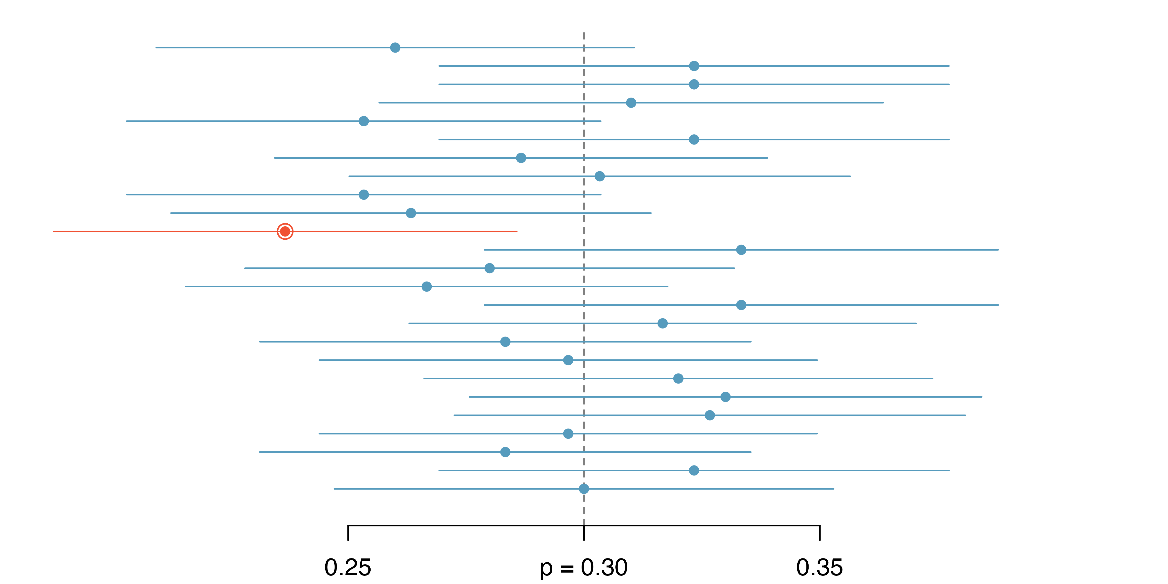
Figure 13.11: Twenty-five samples of size n=300 were collected from a population with p=0.30. For each sample, a confidence interval was created to try to capture the true proportion p. However, 1 of these 25 intervals did not capture p=0.30.
- This is one of the most common errors: while it might be useful to think of it as a probability, the confidence level only quantifies how plausible it is that the parameter is in the interval.
- Our intervals say nothing about the confidence of capturing individual observations, a proportion of the observations, or about capturing point estimates.
- Confidence intervals provide an interval estimate for and attempt to capture population parameters.
Hypothesis test
First draft
Let’s setup a hypothesis to test if stents work to reduce the risk of a stroke.
\(H_{0}\): Stents don’t work
\(H_{A}\): Stents reduce the risk of a stroke
Hypothesis test
Revision 1:
Making it a statement about two groups
\(H_{0}\): Patients who have a stent have the same risk of a stroke as patients who don’t have a stent
\(H_{A}\): Patients who have a stent have lower risk of a stroke as patients who don’t have a stent
Hypothesis test
Revision 2:
Make it a statement using summary statistics and removing the directionality of the hypothesis
\(H_{0}\): The proportion of patients with a stent who have a stroke is the same as the proportion of patients without a stent who have a stroke.
\(H_{A}\): The proportion of patients with a stent who have a stroke is different than the proportion of patients without a stent who have a stroke.
Hypothesis test
Revision 3:
Writing it in symbols
Let \(p_{trmt}\) be the proportion of patients with a stent who have a stroke, and \(p_{ctrl}\) be the proportion of patients without a stent who have a stroke
\(H_{0}: p_{trmt} = p_{ctrl}\)
\(H_{A}: p_{trmt} \neq p_{ctrl}\)
Hypothesis test
Revision 3.5:
Rewriting as a difference in parameters
Let \(p_{trmt}\) be the proportion of patients with a stent who have a stroke, and \(p_{ctrl}\) be the proportion of patients without a stent who have a stroke
\(H_{0}: p_{trmt} - p_{ctrl} = 0\)
\(H_{A}: p_{trmt} - p_{ctrl} \neq 0\)
Using the Normal model
Now we have a statistic (difference in proportions \(p_{trmt} - p_{ctrl}\)) and a null value of 0 to compare it to.
The conditions necessary to ensure the point estimate is nearly normal have been verified for you.
The estimate’s standard error is \(SE = 0.028\) has been calculated for you as well.
Calculating a test statistic & p-value
\[ Z = \frac{\mbox{point estimate - null value}}{SE}\]
\[ Z = \frac{(p_{trmt} - p_{ctrl}) - 0}{SE_{p_{trmt} - p_{ctrl}}} = \frac{.090}{.028} = 3.21 \]
\[ P(Z > 3.2) = .00068 \qquad \mbox{ (the p-value)}\]
If the true difference in proportions was 0, then the probability of observing a difference of 0.09 due to random chance is 0.00068.
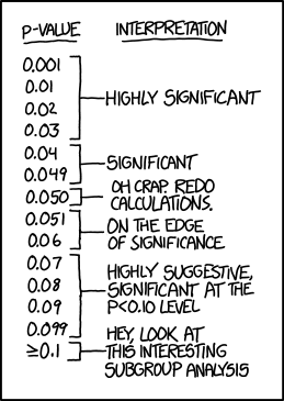
https://xkcd.com/1478/
Using Confidence Intervals to test a hypothesis
We are 95% confident that implanting a stent in a stroke patient’s brain increased the risk of stroke within 30 days by a rate of 0.035 to 0.145.
Since the interval does not contain the null hypothesized value of 0 (is completely above 0), it means the data provide convincing evidence that the stent used in the study changed the risk of stroke within 30 days