Describing Relationships between variables
2025-09-17
Q ~ C
Quantitative Response vs Categorical Explanatory
n, nean, median, sd, IQR of the quantitative variable for each level of the categorical level.
Show the code
# A tibble: 3 × 6
  species       n  mean median    sd   IQR
  <fct>     <int> <dbl>  <dbl> <dbl> <dbl>
1 Adelie      152  18.3   18.4 1.22   1.5
2 Chinstrap    68  18.4   18.4 1.14   1.90
3 Gentoo      124  15.0   15   0.981  1.5
Gentoo penguins have lower average bill depth compared to Adelie or Chinstrap (15.0mm vs 18.3 and 18.4mm respectively). Chinstrap however have a larger IQR at 1.9 compared to 1.5 for the others.
Similarly nice tables, but defaults to median and IQR.
Have to manually specify you want mean & sd.
Overlaid density plots
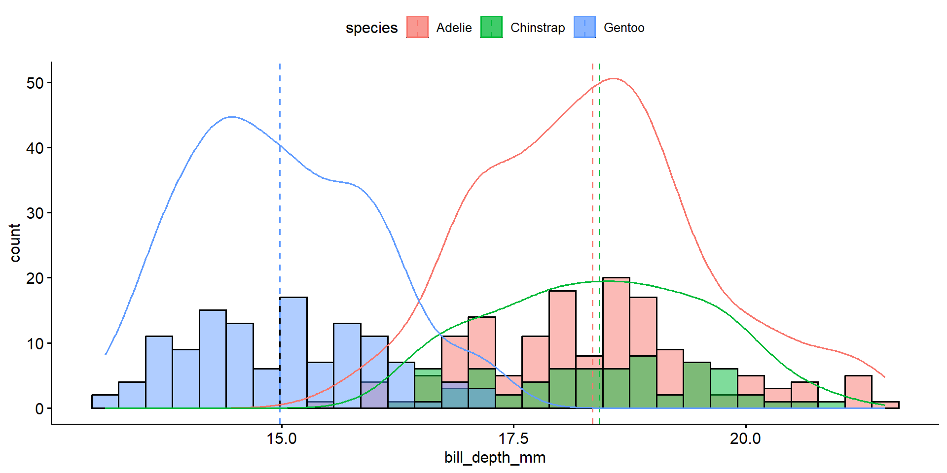
The distribution of bill depth are fairly normal for each species, with some higher end values causing a slight right skew for Adelie and Gentoo.
More code but nice alternative to violins.
Show the code
library(ggdist) # for the "half-violin" plot (stat_slab)
ggplot(pen, aes(x=bill_depth_mm, y=species, fill=species)) +
      stat_slab(alpha=.5, justification = 0) +
      geom_boxplot(width = .2,  outlier.shape = NA) +
      geom_jitter(alpha = 0.5, height = 0.05) +
      stat_summary(fun="mean", geom="point", col="red", size=4, pch=17) +
      theme_bw() +
      labs(x="Bill depth (mm)", y = "Species") +
      theme(legend.position = "none")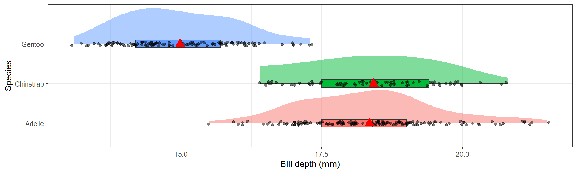
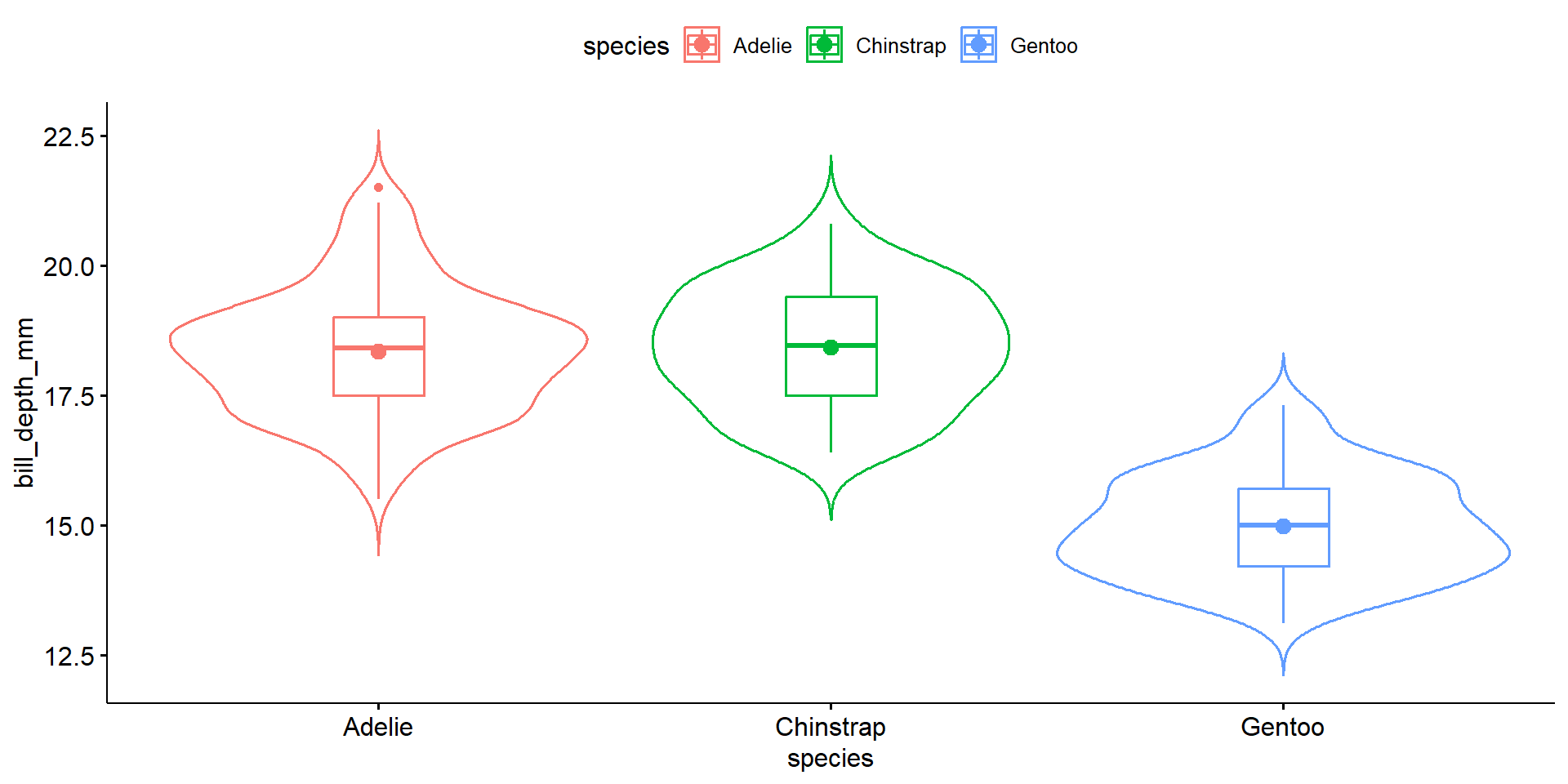
Discuss shape, spread and center using comparative language.
The distribution of bill depth are fairly normal for each species, with some higher end values causing a slight right skew for Adelie and Gentoo. Gentoo penguins have lower average bill depth compared to Adelie or Chinstrap (15.0mm vs 18.3 and 18.4mm respectively). Chinstrap however have a larger IQR at 1.9 compared to 1.5 for the others.
Q ~ Q
Quantitative Response vs Quantitative Explanatory
[1] 0.8712018The correlation coefficient \(r\) is a measure of the strength and direction of a linear relationship between two variables.
- \(|r| > 0.6\) Strong relationship
- \(0.4 \leq |r| < 0.6\) Moderate relationship
- \(|r| < 0.4\) Weak to no relationship
Note: These values are guidelines and subject to variability within different disciplines ref
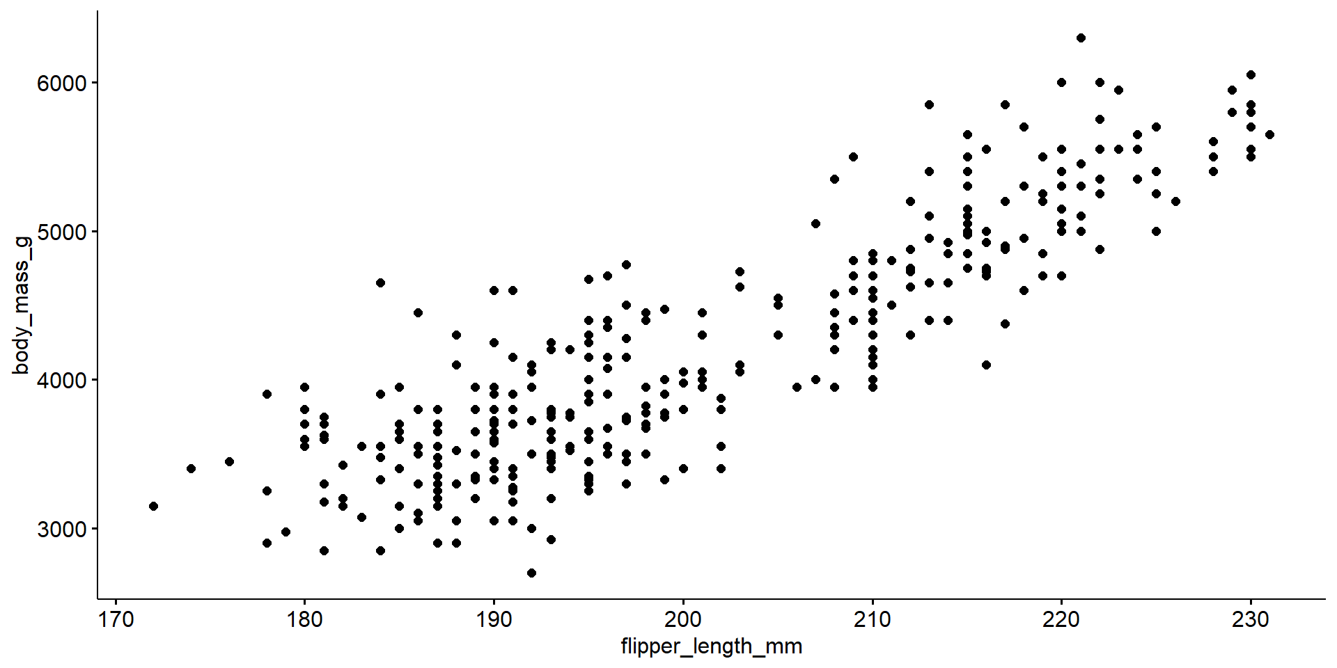
The relationship between flipper length and body mass in penguins is relatively linear, but there may be possible clustering on a third variable. There appears to be two groups below and above a flipper length of about 205mm.
Must include the direction (positive or negative), the strength quantified using \(r\), and the form (linear vs non-linear)
The penguin flipper length (mm) has a strong, positive, and reasonably linear correlation with body mass (g), r=0.87.
C ~ C
Categorical Response vs Categorical Explanatory
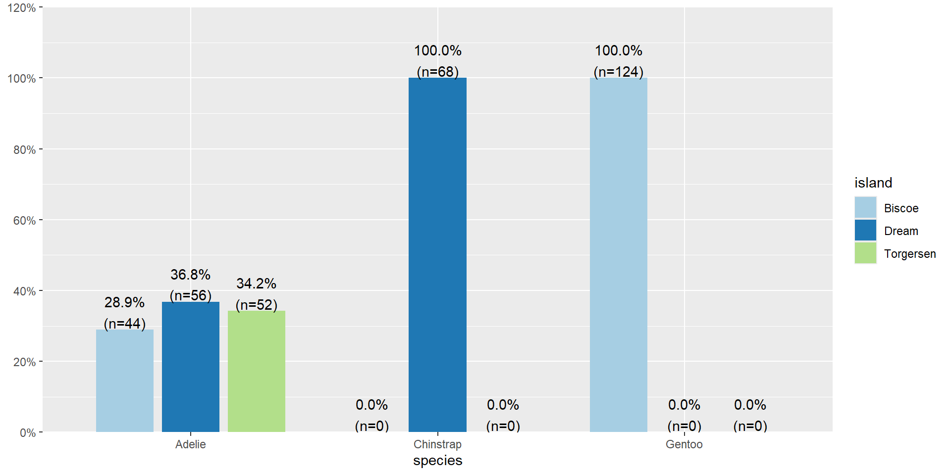
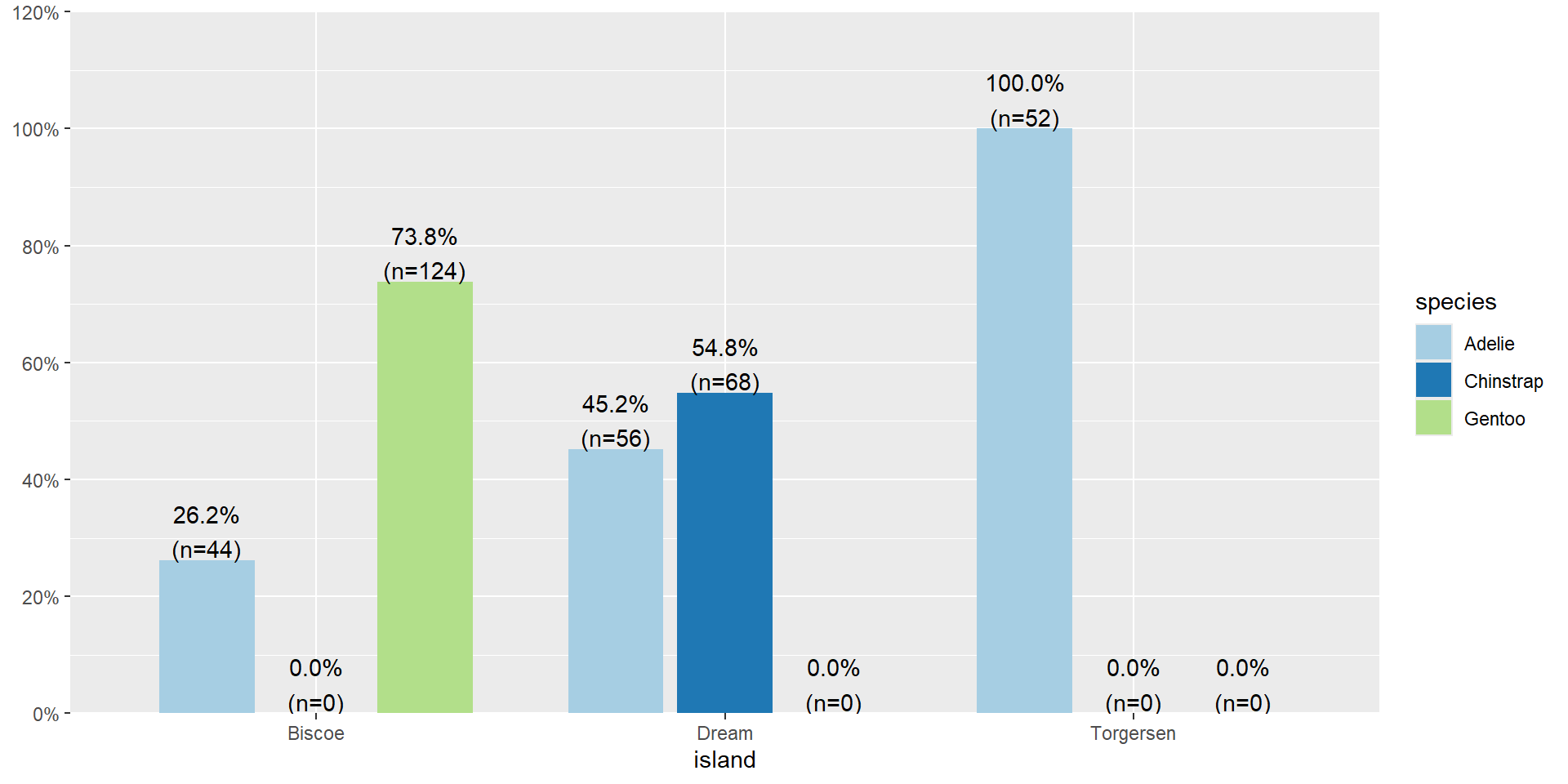
- All of the 52 penguins on Torgersen island are the Adelie species.
- 74% of penguins on Biscoe island are Gentoo.
Watch your margins
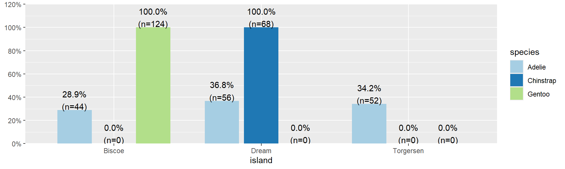
Row Percents
            Biscoe Dream Torgersen
  Adelie      0.29  0.37      0.34
  Chinstrap   0.00  1.00      0.00
  Gentoo      1.00  0.00      0.00
29% of Adelie penguins are on Biscoe Island.
Distribution of Islands within each species
Distribution of islands for each species
29% of Adelie penguins are on Biscoe Island.
